Performance¶

Overview¶

Both models perform better (on average) than the NBA’s model, with a particular advantage in early game prediction.
The Lifelines model outperforms the XGBoost model.

For generating player ratings, we will use the Lifelines model.

Performance¶

Important

At this time the models have been trained on data from the 2005-06 through the 2019-20 seasons (pre-bubble). The final build dataset had 10 765 games with 1 188 655 rows; the tuning/stopping datasets had 3 589 games with 396 863 rows; the holdout dataset had 3 589 games with 396 189 rows.

Figure 1 shows the AUROC over game-time for each model.

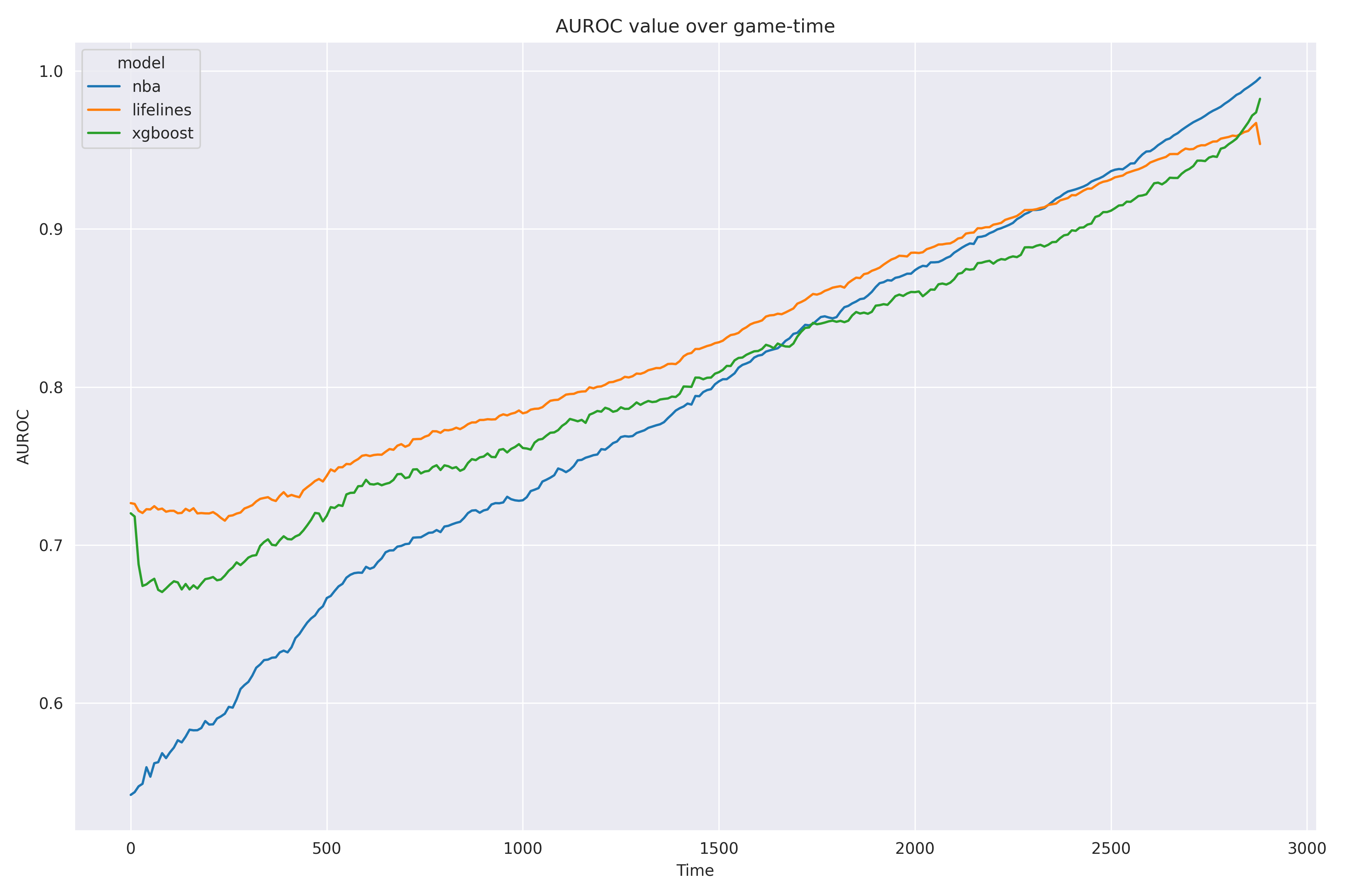
Figure 2 directly shows the AUROC lift of each survival model against the NBA win probability model.

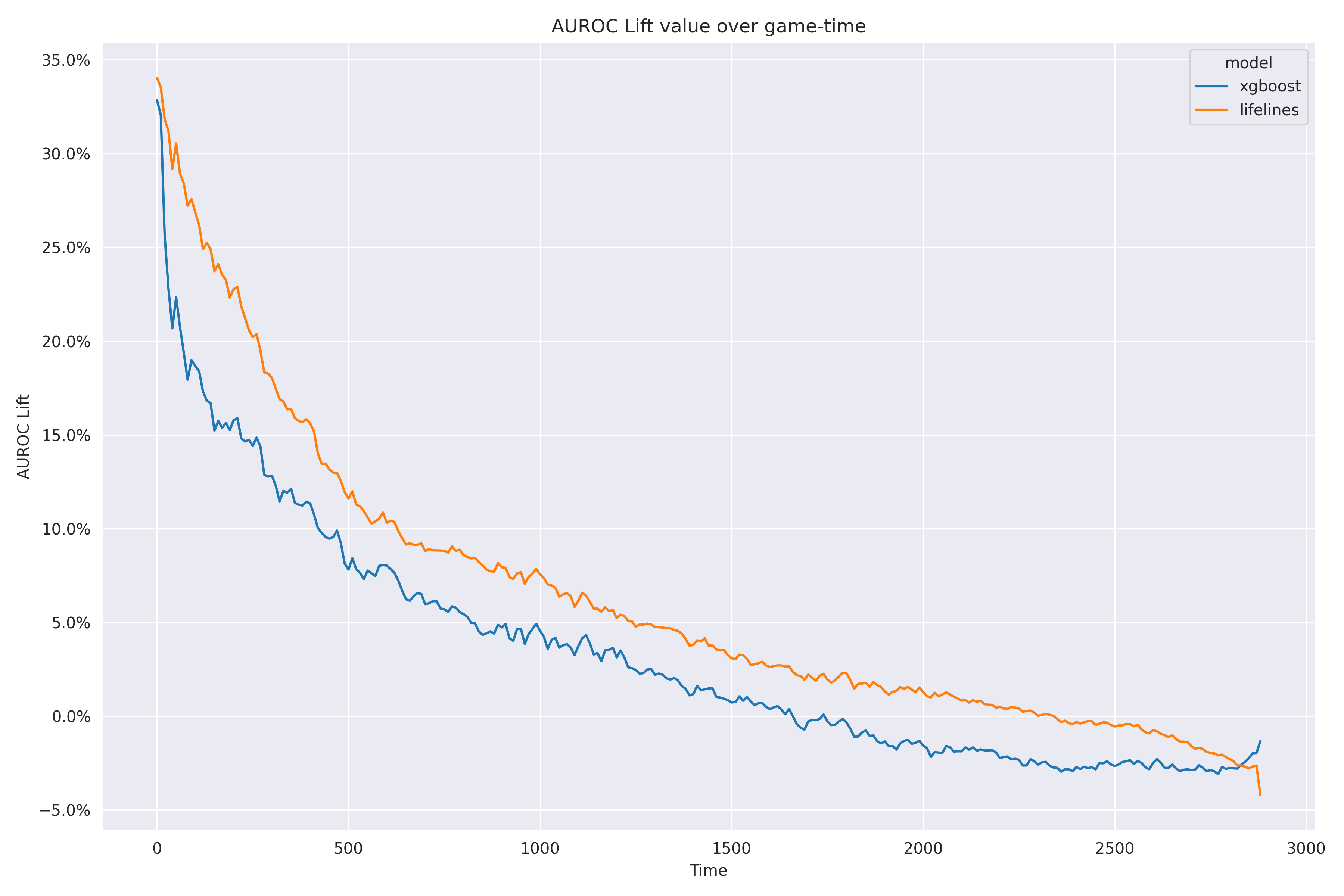
Overall, the average AUROC lift for each model is summarized below:

Model	Average AUROC	Percentage lift over NBA model
XGBoost	0.808	3.3%
Lifelines	0.831	6.315%

Model Characteristics¶

Lifelines¶

Figure 3 shows the hyperparameter tuning results for the lifelines model. The tuning was done using 1 000 evaluations.

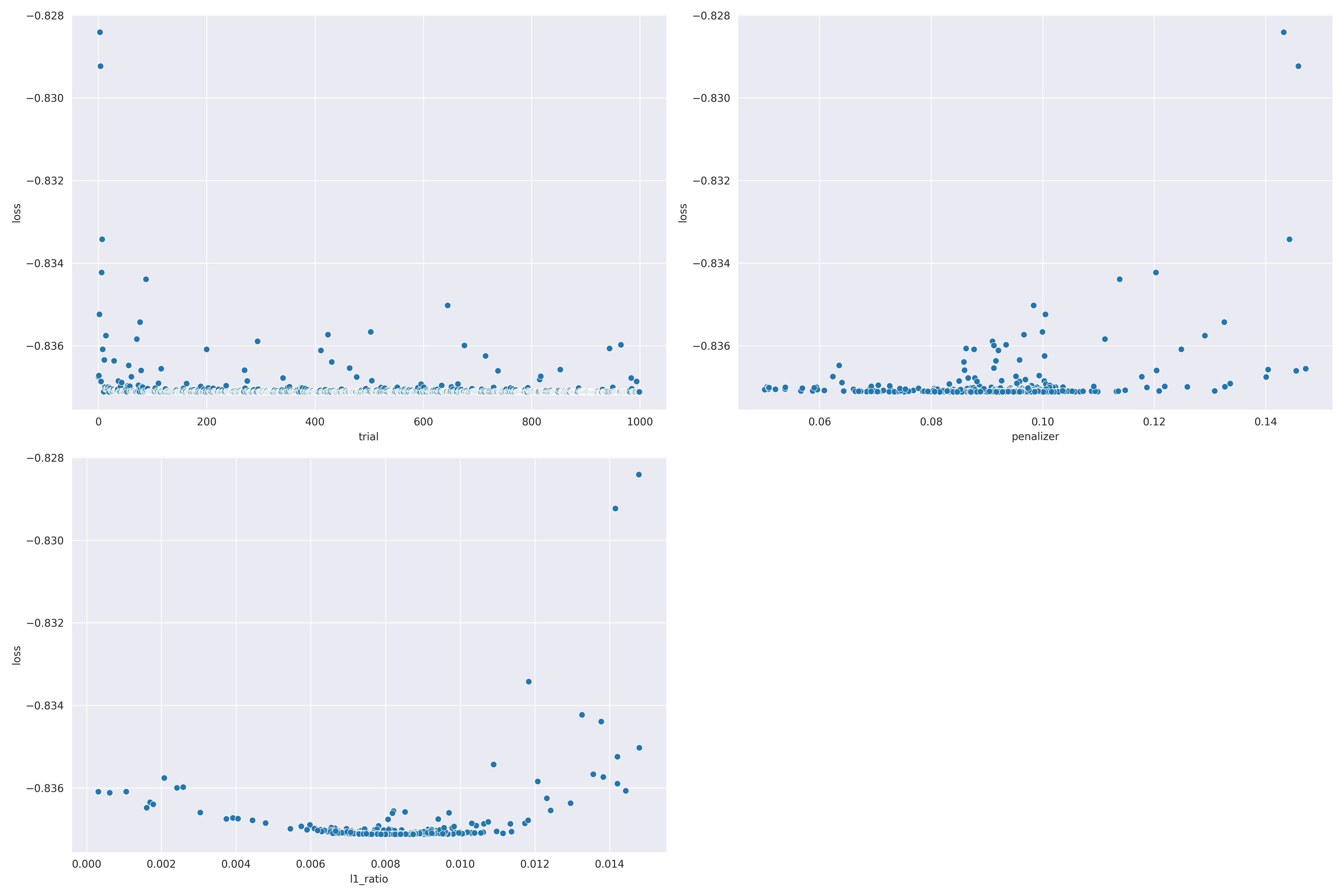
Tuning led to the following final hyperparameters:

Hyperparameter	Value
`l1_ratio`	0.007994777879269076
`penalizer`	0.09127606625097757

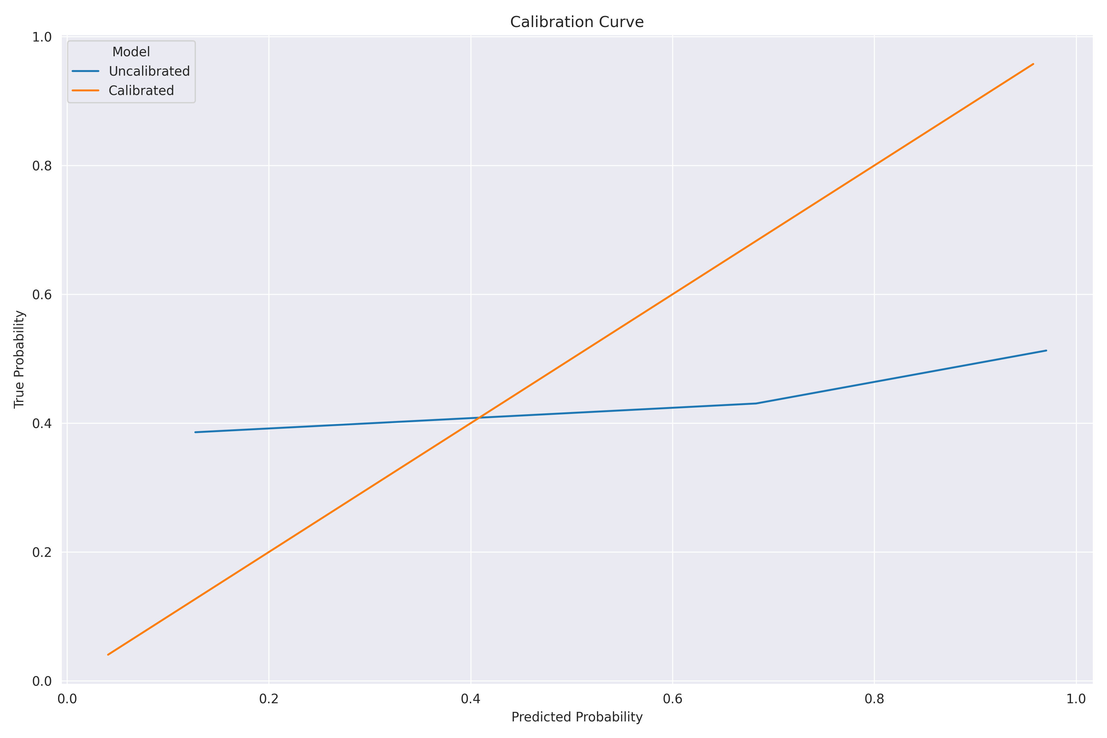
Isotonic regression produced the following calibration plot:

XGBoost¶

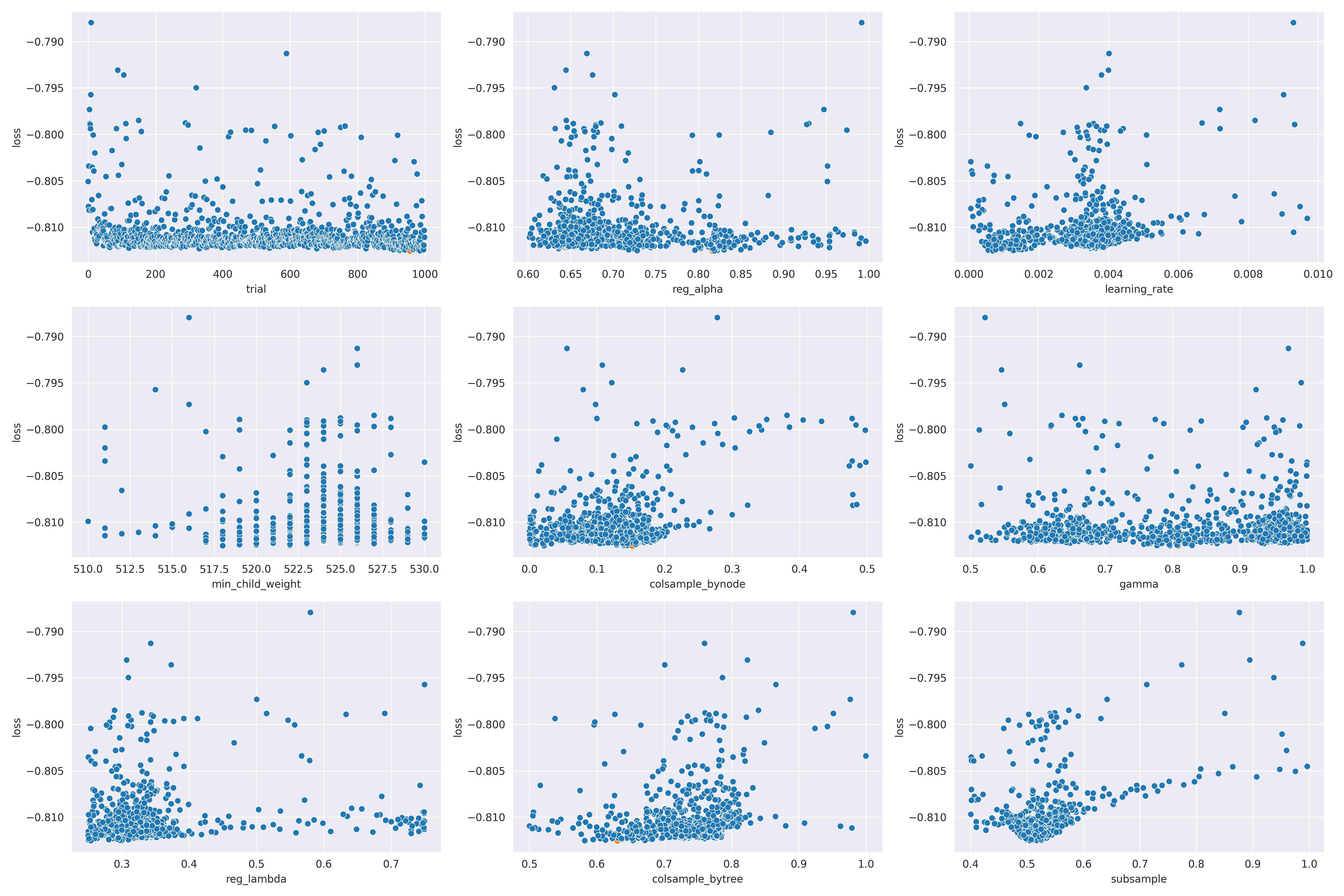
Figure 5 shows the hyperparameter tuning results for the xgboost model. The tuning was done using 1 000 evaluations.

Tuning led to the following hyperparameters:

Hyperparameter	Value
`colsample_bylevel`	1
`colsample_bynode`	0.15221691031911938
`colsample_bytree`	0.6308916896893483
`gamma`	0.8083332824721229
`learning_rate`	0.0006959999989275942
`max_delta_step`	1
`max_depth`	4
`min_child_weight`	518
`monotone_constraints`	(0, 0, 0, 0, 0, 0, 0, 0, 0, 0, 0, 1, 0, 0)
`reg_alpha`	0.8166483270728037
`reg_lambda`	0.2533343088849453
`subsample`	0.5043820990853263

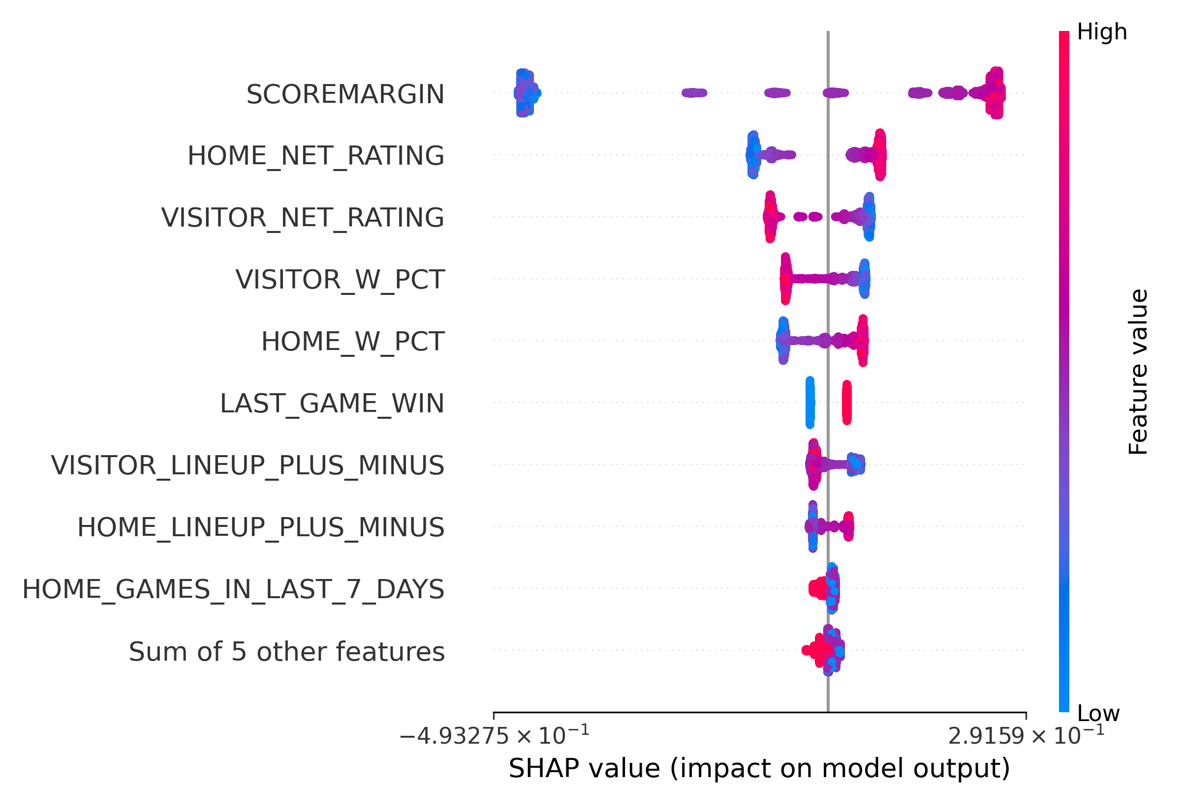
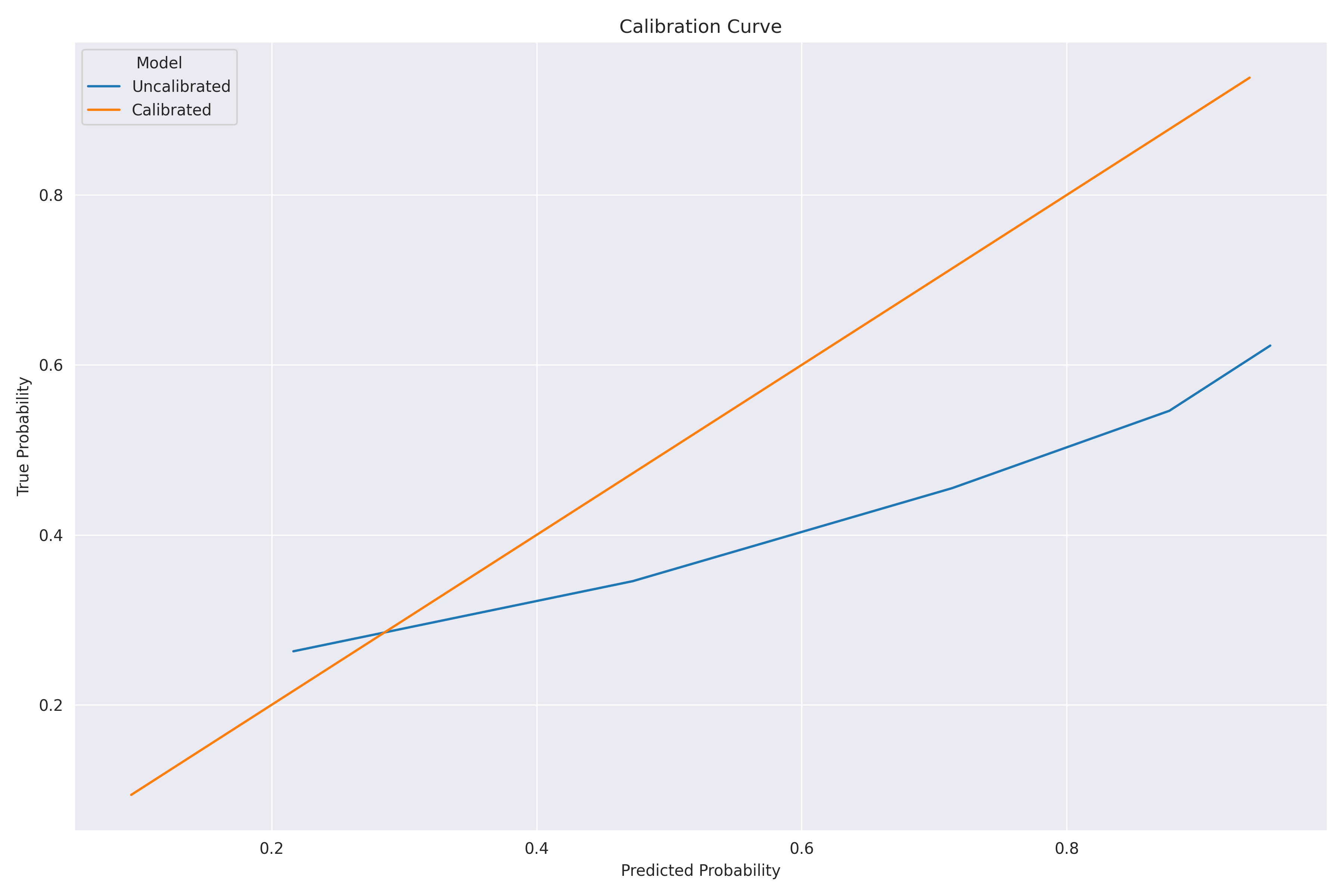
Isotonic regression produced the following calibration plot:

Since XGBoost doesn’t produce directly interpretable coefficients like a linear model, we will use SHAP to produce feature importances: